What is Backpropagation
Imagine teaching a robot to distinguish between cats and other animals, each time it makes a mistake you adjust its thought process slightly, to make it better at this task. In artificial intelligence, this fine-tuning is achieved through an algorithm known as backpropagation. It’s a method that iteratively adjusts a neural network’s parameters, steering it towards higher accuracy.
But how does backpropagation know which way to adjust? It uses calculus, specifically by finding the gradient with respect to a loss function. This gradient acts like a compass, pointing towards the direction where the network’s output or predictions become more accurate. This process is not just limited to neural networks; it’s a general technique applicable to various mathematical expressions, making it a universal tool in machine learning.
Since its inception, backpropagation has been pivotal in the resurgence and success of neural networks, marking a key milestone in the AI revolution. The upcoming sections, will explore the building blocks of neural networks, the intuition and math behind backpropagation and it’s application in training neural networks.
Artificial Neural Networks
Artificial neural networks (ANNs) are designed to emulate the way biological neurons in the human brain process information. These networks comprise interconnected nodes or neurons arranged in layers, communicating through connections akin to biological synapses. Each neuron in an ANN receives and processes data, contributing to the overall task of the network, such as classification or pattern recognition. By mimicking these biological processes, ANNs harness the complex, adaptive nature of the human brain to solve diverse computational problems.
Understanding the Neural Network Architecture
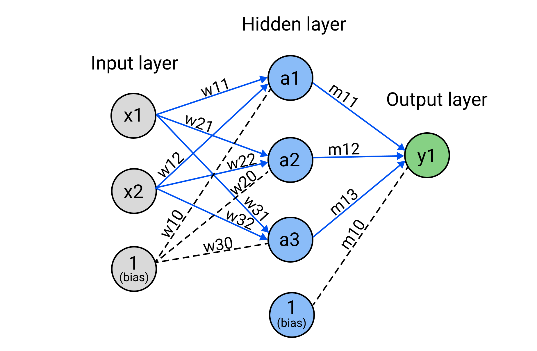
Before going into the details of backpropagation, it’s essential to grasp how neural nets are structured and the concept of forward propagation. Consider a simple neural network that consists of a few layers:
- Input Layer: This is where the network takes in data. The nodes \(x1\) and \(x2\) represent the features of this input data. A bias unit is often included in this layer to account for offset in the decision boundary.
- Hidden Layer: In this layer, the input data is processed by the neurons \(a1\), \(a2\) and \(a3\). Each connection from the input to the hidden layer is weighted \(W_{ij}\) , the strength of these weights signifies the importance of the input values to the neurons.
- Activation Function: Each neuron in the hidden layer processes input weighted data by summing them and applying an activation function. This aspect is crucial as these functions introduce non-linearity in the network and enable the network to capture complex patterns. Without them, the neural network would become a linear regressor, regardless of how many layers we add.
- Output Layer: The neuron \(y1\) receives processed information from the hidden layer neurons and through weighted connections \(M_{1j}\), generates the final output after applying an activation function.
Diving Deeper into Activation Functions
While we’ve previously mentioned how activation functions introduce non-linearity, let’s explore specific use cases and characteristics of common functions such as sigmoid, Tanh and ReLU.
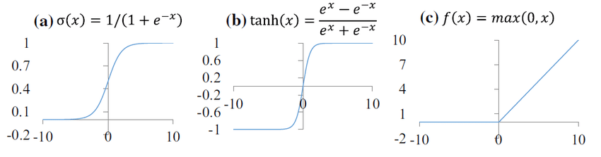
Sigmoid
The sigmoid function’s smooth S-shaped curve allows it to approximate binary functions closely. It is continuous and differentiable, which makes it suitable for gradient-based optimisation methods. However, it can result in vanishing gradients, where gradients shrink and their derivates become tiny, resulting in negligible parameter updates and effectively halting the network from further training. This is especially problematic in deep networks with many layers.
Tanh
Often used in hidden layers where data is zero-centered; it helps in transitioning data effectively through layers without shifting the mean, which can accelerate learning. However, Tanh also suffers from vanishing gradients, although to a lesser extent than the sigmoid function due to its symmetric output range. This range can help with convergence during training because it tends to centre the output of the neurons. Neurons in later layers of deep networks start with activations that are not too small or too large, which can lead to more stable learning in the early stages.
ReLU
ReLU, short for Rectified Linear Unit, is widely used in deep neural networks due to its ability to facilitate faster and more effective learning, particularly in layers deep within the network. It directly counters the vanishing gradient problem by allowing positive gradients to flow through without change, which accelerates convergence during training. Despite its advantages, ReLU can be susceptible to “neuron death” during training, where neurons may stop participating in the data transformation process if their gradients reach zero, known as the “dying ReLU” issue.
Demonstrating a Forward Pass
Going back to our original diagram and using the concepts covered so far, namely layers, weights, biases and activation functions we will now complete a forward pass to obtain the output of our neural network using the inputs, network parameters and sigmoid activation function.
- Inputs: \(x1 = 1, x2 = -1\)
| Parameter | Value |
|---|---|
| \(w11\) | 1 |
| \(w21\) | 0.5 |
| \(w12\) | -0.5 |
| \(w22\) | 1 |
| \(w31\) | 0 |
| \(w32\) | 0.5 |
| \(m11\) | 0.25 |
| \(m12\) | -1 |
| \(m13\) | 1 |
| \(w10\) | 0.10 |
| \(w20\) | 0.20 |
| \(w30\) | -0.1 |
| \(m10\) | 1 |
- \(f(z) \frac 1 {1+e^{-z}}\)
\(a_1 = f(x1 \cdot w11 + x2 \cdot w12 + w10) = 0.83\)
\(a_2 = f(x1 \cdot w21 + x2 \cdot w22 + w20) = 0.430\)
\(a_3 = f(x1 \cdot w31 + x2 \cdot w32 + w30) = 0.354\)
\(y_1 = f(a1 \cdot m11 + a2 \cdot m12 + a3 \cdot m13 + m10) = 0.532\)
Loss Function
Now that we know the output from our network we need to evaluate the accuracy of its prediction, quantifying how close we are to the true value. This is where the loss function comes into play. The loss function measures the disparity between the predicted output of the neural network and the actual output. By calculating this difference, we can determine how well the network is performing and use it to guide the backpropagation process for further improvement. For this example, we will use mean squared error as our loss.
\(\text{MSE} = \frac{1}{N} \sum_{i=1}^{N} (Y_i - \hat{Y}_i)^2\)
Where:
\(N\) is the number of samples
\(Y_i\) is the observed value
\(\hat Y_i\) is the predicted value
For instance, if the actual value of y is 1 and we know that our neural network predicted 0.532 then we can find the error associated with this output:
\(MSE = (1 - 0.532)^2 = 0.219\)
In this case, we consider the number of samples to be 1, but this usually won’t be the case as the error will be averaged over many samples in the training set.
Other Loss Functions
Selecting an appropriate loss function is another important consideration when training a neural network, this usually depends on the type of task and has significant implications for the convergence and performance of the neural network. Here are a few other common loss functions:
Mean Absolute Error (MAE)
Use Cases: Regression tasks.
Advantages: Robust to outliers as errors are not squared in the calculation.
Disadvantages: Because the errors are not squared this can understate the impact of large errors, which may not always be desirable.
Mathematical Expression: \(MAE = \frac 1N \sum_{i=1}^{N} |y_i -\hat y|\)
Binary Cross Entropy (Log Loss)
Use Cases: Binary classification tasks.
Advantages: Well suited for measuring the performance of a classification model whose output is a probability value between 0 and 1.
Disadvantages: Can be sensitive to imbalanced datasets where the number of instances of a class significantly outnumber the other.
Mathematical Expression: \(L_{\text{BCE}} = -\frac{1}{N} \sum_{i=1}^{N} \left [(Y_i \cdot \log\hat{Y}_i + (1 - Y_i) \cdot \log(1 - \hat{Y}_i)) \right]\)
Categorical Cross-Entropy
Use Cases: Multi-class classification tasks.
Advantages: Generalises binary cross-entropy to multiple classes and is effective when each sample belongs to exactly one class.
Disadvantages: Like binary cross-entropy, it can be sensitive to imbalanced datasets.
Mathematical Expression: \(L_{CCE} = \frac 1N \sum_{i=1}^{N} \sum_{c=1}^{M}y_{ic}\cdot log(\hat y_{ic})\)
Where: \(M\) is the number of classes
Hinge Loss
Use Cases: Binary classification tasks, especially for SVMs (support vector machines).
Advantages: It encourages the model to not only make the correct prediction but also to make it with high confidence.
Disadvantages: Not suitable for probability estimates, as it does not model probability distributions.
Mathematical Expression: \(L_{Hinge} = \frac 1N \sum_{i=1}^{N} max(0, 1 - y_i \cdot \hat y_i)\)
Learning by Reversing
Now that we have a good idea of how well our neural network is performing via the loss function, we can focus on gradually improving it’s performance. This is where backpropagation comes into play. Backpropagation is a methodical way of adjusting the weights in our network to minimise the loss. By calculating how the loss changes with respect to each weight, we can adjust the weights in the direction that reduces the loss, iteratively enhancing the network’s predictions. By repeatedly applying forward and backpropagation across multiple iterations over the entire dataset, the network learns a more precise model of the input-output relationship. Ultimately, this allows the network to incrementally capture the underlying patterns in the data, leading to more accurate predictions.
The Chain Rule
The chain rule from calculus is expressed as:
\[ \frac {dy}{dx} = \frac {dy}{du} \cdot \frac {du}{dx} \]
It helps us understand how two rates of change are related. Imagine \(y\) depends on \(u\) and \(u\) depends on \(x\). If you know how quickly \(y\) changes with \(u\) and how quickly \(u\) changes with \(x\), then the chain rule allows us to multiply these two rates to find out the rate of change of \(y\) with respect to \(x\). It’s like figuring out the total effect on \(y\) when \(x\) changes, by linking their relationship through a common variable \(u\).
Computing Gradients
With the chain rule in mind, we can calculate the gradient of the loss function with respect to each weight in the neural network. Essentially, backpropagation reverses the flow of computation in the neural network. Starting from the output it propagates the error back through the network, layer by layer. At each neuron, the chain rule is used to find out to what extent weights and biases need to be adjusted to reduce the error, linking the rate of change of the error with respect to the output (which we want to minimise) to the rate of change of the output with respect to the weights and biases (which we can control). This linkage allows us to backpropagate the error and update our weights to improve our model.
For instance, applying the chain rule for the weight \(m11\) gives us the expression:
\[ \frac{\partial \theta}{\partial m11} = \frac{\partial \theta}{\partial y1} \cdot \frac{\partial y1}{\partial net} \cdot \frac{\partial net}{\partial m11} \]
Where:
- \(y1 = f(net)\)
- \(net = a1 \cdot m11 + a2 \cdot m12 + a3 \cdot m13 + m10\)
- \(\theta\) is the loss function
The weight \(m11\) directly influences the output of the neural network by scaling the activation \(a1\) from the hidden layer before it contributes to the output neuron \(y1\). In essence, \(m11\) modulates how much \(a1\) impacts the final prediction. By adjusting \(m11\), we can control the strength of this influence. During the training process, we seek to find the optimal value of \(m11\) that minimises the loss function.
Going further back in the network, we can derive the expression for \(w22\) too:
\(\frac{\partial \theta}{\partial w22} = \frac{\partial \theta}{\partial y1} \cdot \frac{\partial y1}{\partial f(a2)} \cdot \frac{\partial f(a2)}{\partial a2} \cdot \frac{\partial a2}{\partial w22}\)
The weight \(w22\) plays a pivotal role in determining the output of a neural network by influencing the activation of neuron \(a2\) in the hidden layer. A change in \(w22\) alters the weighted input to \(a2\), which, due to the sigmoid function, significantly affects the \(a2\) activation level. This change is then carried forward, impacting the input and, subsequently, the activation of the output neuron \(y1\). Since the output \(y1\) is a result of applying the sigmoid function to its total input, any modification in \(w22\) leads to a non-linear alteration in \(y1\). This alteration cascades to affect the network’s loss \(\theta\), akin to a domino effect, where adjusting the initial element \(w22\), steers the network towards a lower loss and improved performance.
Updating Parameters
The computed gradients are used to make small adjustments to the weights and biases, a process guided by the learning rate, a hyperparameter that controls the size of these adjustments. This step is crucial; too large a learning rate can lead to overshooting the minimum of the loss function, while too small a learning rate can cause the training process to stall.
Our update equation for \(w11\) becomes:
\(m11 = m11 - \alpha \left[\frac{\partial \theta}{\partial y1} \cdot \frac{\partial y1}{\partial net} \cdot \frac{\partial net}{\partial m11} \right]\)
Where:
- \(\alpha\) is the learning rate
The partial derivative \(\frac{\partial \theta}{\partial m11}\) encapsulates the sensitivity of the loss function to changes in \(m11\). A negative derivative suggests increasing \(m11\) reduces the loss, while a positive one implies the opposite. The update rule in training uses this derivative, along with the learning rate \(\alpha\) to adjust \(m11\) effectively. This adjustment is in the opposite direction of the gradient to minimise the loss. Imagine the loss function as a hill; moving against the gradient guides us downhill towards the loss minimum. Through iterative updates, the network “learns” by tuning \(m11\) to enhance prediction accuracy.